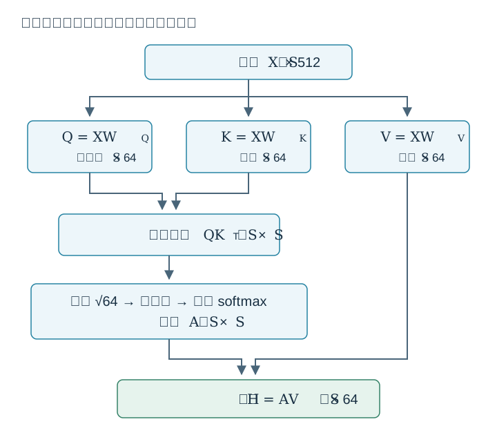
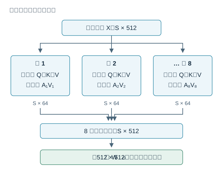
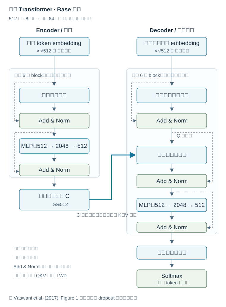
文中以《Attention Is All You Need》的原始架构为主，并在相关位置说明它与 GPT-2 的区别。除特别说明外，省略 batch 维度，以单条序列为单位讨论。

1. 词表大小、序列长度与隐藏维度

计算中需要区分三个量：

“100k 上下文”说的是可容纳的 token 数量上限。实际输入只有 1,000 个 token 时，当前序列长度就是 1,000。词表里的其他 token 不会因此各占一个注意力位置。

分词器有不同设计。BPE 等子词方法会从较小单位出发，把频繁出现的组合合并为 token。词表不必收录每一个完整单词：一个没见过的长词，仍可能被拆成已有片段。采用完整字节覆盖的方法可以进一步用字节表示输入；其他方法可能需要未知 token。

词表大小通常通过实验和预算取舍。词表小，文字可能切得更碎；词表大，embedding 和词表输出层更大，一些罕见 token 也更难获得充分训练。在模型训练完成后，词表和编号映射通常保持固定。

2. Token embedding

每个 token 有一个编号。编号用于查表，其大小和相邻关系不表示语义关系。设 embedding 表为：

根据当前序列的 token 编号，从 \(E\) 中取出对应的 \(S\) 行，按序列顺序排列，得到：

同一个 token 出现多次，就会重复取出同一行，放到不同的序列位置。向量的数值通过训练确定，单个分量通常没有明确的语义标签，信息可以由多个分量共同表示。

从头训练时，embedding 权重通常随机初始化，然后与整个网络一起优化。训练好的模型直接加载这张表。同一个 token 的初始向量相同，但后续会根据上下文产生不同状态。

这里需要区分两类量：参数是模型保存的可训练数值；状态是给定输入后计算出的中间结果。 \(E\) 是参数矩阵，查表得到的 \(X_{\mathrm{token}}\) 是当前输入的表示。

3. 位置编码

仅有 token embedding 还没有显式表示顺序。原论文将每个位置的编码与该位置的 token embedding 相加。设当前序列的位置编码矩阵为 \(P\)，则：

这里的 \(\sqrt{d}\) 是原论文采用的 embedding 缩放系数。相加按元素进行，结果的尺寸不变。token 编号决定从 embedding 表取哪一行；位置编号决定使用哪个位置向量。词表大小与可表示的位置数量没有必要相等。

同一个 token 出现在不同位置时，token embedding 相同，位置编码不同。相加后，网络便能利用位置差异区分不同的排列顺序。

原始 Transformer 使用固定的正弦、余弦位置编码，不同分量具有不同频率。GPT-2 使用可学习的绝对位置表。前者的位置向量由公式生成，后者的位置向量参与训练。[1, 2]

下文用 \(X\) 表示送入某个注意力模块的状态：第一层接收上述输入，后续层接收上一层处理后的结果。为具体说明尺寸，采用原论文 base 配置：\(d=512\)，8 个注意力头，每头 64 维。

4. 查询、键和值

一个注意力头有三个可训练的投影矩阵：

它们分别作用于同一个输入矩阵：

因此，\(Q\)、\(K\)、\(V\) 都是 \(S\times64\) 的矩阵。它们的每一行对应一个序列位置：

“某个位置的 query”指 \(Q\) 中对应的那一行，是一个向量。同一个头中，所有位置都使用同一套 \(W_{Q}\)。矩阵乘法将每一行分别投影，再把结果按行排列；每个位置并没有独立的投影参数。\(K\) 和 \(V\) 同理。

\(K\) 用于计算匹配分数，\(V\) 用于后续的加权求和。分别使用两个可训练投影，使模型可以独立调整匹配所需的特征和需要传递的内容。

5. 注意力权重与加权求和

先计算所有接收位置与源位置之间的匹配分数：

上标 \(\mathsf{T}\) 表示转置。尺寸关系为：

这个分数矩阵的每一行对应一个接收位置，每一列对应一个源位置。\(Q\) 的某一行与 \(K\) 的每一行分别做点积，得到 \(S\) 个分数。点积内部对向量分量求和，不同源位置的分数则分别保留。

设遮挡矩阵为 \(M\)：允许读取的位置取 0，禁止读取的位置取负无穷。注意力权重为：

缩放用于控制点积分数的尺度。softmax 按行执行，将每行分数转换为非负、总和为 1 的权重；被遮挡的位置权重为零。这里假设每行至少有一个允许读取的位置。

随后用权重对值向量进行混合：

\(H\) 是这个头的输出。它的每一行，是 \(V\) 中各行按对应注意力权重形成的加权和。

因此，不同位置的信息通过两步影响输出：其他位置的键向量影响读取权重，其他位置的值向量参与输出的加权求和。

这也解释了同一个 token 如何在不同语境下产生不同表示。即使某个位置的初始表示相同，周围位置的键和值不同，注意力输出也可以不同。新状态继续进入后续层，但不会直接写回 embedding 表；训练时更新参数表的是反向传播得到的梯度。

将输入依赖关系显式写出：

给定 \(A\) 后，加权求和对 \(V\) 是线性的；整体注意力操作则是非线性的，因为 \(A\) 也由输入计算得到。注意力权重描述这一层的信息读取，不能单独解释模型的最终判断。

6. 多头注意力

每个头都读取完整的输入矩阵，再通过各自的投影生成 \(Q\)、\(K\)、\(V\)。每个 \(512\times64\) 投影矩阵都能将全部 512 个输入分量混合到 64 个输出分量中，并不是只读取输入的一部分。

多个头的投影矩阵可以并排放成一个大矩阵，一次乘法算完，再将结果拆成各头。这与分别投影在数学上等价。

随后，各头分别计算自己的注意力权重矩阵。这样，同一个接收位置可以通过不同的头，使用不同权重读取信息。如果把所有头的通道合起来只计算一次点积和 softmax，就只得到一套位置权重。

设八个头的输出为 \(H_{1},\ldots,H_{8}\)。沿列方向拼接，再经过注意力输出投影：

拼接结果和 \(O\) 的尺寸都是 \(S\times512\)。\(W_{O}\) 允许不同头的输出相互混合。标准多头注意力会使用全部头的输出，各头在共同损失下训练，其功能可能互补，也可能重叠。

同一层各头的注意力计算不等待其他头的结果；下一层则可以基于上一层已经整合的信息继续处理。头数增加并行读取方式，深度增加有先后依赖的处理轮次。 若隐藏维度固定，更多头通常意味着每头更窄，并不自动带来更强能力。

7. 残差连接与 MLP

注意力输出 \(O\) 与输入 \(X\) 尺寸相同。原论文先将它们相加，再做层归一化：

在归一化之前，残差连接 \(X+O\) 提供了一条系数为 1 的直接通路。当更新量 \(O\) 接近零时，相加结果接近 \(X\)。这并不表示经过 LayerNorm 后的整个模块严格等于恒等变换。

用标量形式说明残差本身的梯度：

导数中的 1 对应直接通路。这有助于梯度传播，但完整网络还包含归一化等操作，不能据此保证梯度始终稳定。其他架构也可以采用缩放或门控残差。

接下来，MLP 对每一行使用同一套参数：

偏置的大小不随输入长度变化。ReLU 提供非线性，否则两个线性变换可以合成一个。MLP 在每个位置内部加工已有信息，本身不跨位置通信。然后再做一次残差与归一化：

这就是原论文 encoder block 的主干。原论文在残差相加前等位置还使用 dropout；为简化表达，这里没有把它写进每条公式。

8. 原始 Transformer：encoder 与 decoder

前面介绍的注意力和 MLP 构成了原始 Transformer 的基本模块。完整模型由 encoder 和 decoder 两部分组成，各有六个串联的 block，同一部分内各层结构相同、参数独立。下图根据原论文 Figure 1 重绘，数据从上向下流动。[1]

本文采用的 base 配置为 512 维、8 个头。GPT-2 small 则是 768 维、12 个头和 12 个 decoder-only block；它的 MLP 激活、位置表示和归一化顺序也不同。[2]

为区分两条序列，记原文长度为 \(S_{\mathrm{src}}\)，当前译文前缀长度为 \(S_{\mathrm{tgt}}\)。原文经过六层 encoder，得到：

它保留原文的各个位置，并没有把整句话压成单个向量。Encoder 自注意力允许读取原文的前后位置，但不读取补齐长度用的 padding。

Decoder 的每个 block 则依次包含因果自注意力、交叉注意力和 MLP，每个子层后都有残差相加与归一化。三种注意力的区别如下：

具体地，记 decoder 经过因果自注意力及归一化后的状态为 \(B\)。一个交叉注意力头计算：

这里的投影参数属于该交叉注意力模块，与其他注意力模块的参数独立。各矩阵尺寸为：

因此：

注意力矩阵不必是方阵。输出的每一行仍对应一个译文位置，却已经读取了原文信息。多头合并和输出投影后，残差加回的是 \(B\)，不是 \(C\)。

每个 decoder block 都读取同一个最终 \(C\)，但使用各自的投影参数；不是第几层 decoder 对接第几层 encoder。

9. Decoder-only 模型如何读取输入

Decoder-only 模型可以把任务说明、原文和译文前缀按顺序放进同一条序列。生成译文时，原文已经位于前面，因果自注意力可以读取它。

Self-attention 的 self 指同一组序列表示，不是一个 token 只能读取自己。 同一条序列中不同位置之间的读取仍是自注意力；当查询来自 decoder，而键和值来自独立的 encoder 表示时，才是上一节介绍的交叉注意力。

因此，GPT-2 这类 decoder-only 模型不需要通过额外的交叉注意力接收文字输入。能否做好翻译还取决于训练数据与训练方式，架构提供可行的信息通道，并不自动赋予能力。

10. 推理：预测下一个 token

回到原始 encoder–decoder 模型。Decoder 最后一层的输出经词表投影和 softmax，为每个位置产生一个“下一个 token”的分布：

\(D\) 是 decoder 的最终状态，\(W_{\mathrm{vocab}}\) 是词表输出投影，\(\Pi\) 是预测概率矩阵。词表输出投影与注意力内部的 \(W_{O}\) 作用不同；前者输出词表分数，后者混合多头结果。原论文还让词表输出投影与 embedding 共享权重。

推理从起始标记开始。给定当前前缀，尚未生成的下一个 token 紧跟最后一个位置，因此使用 \(\Pi\) 的最后一行。前面的状态仍参与注意力计算，为最后一个位置提供信息。

选出新 token 后加入前缀，继续预测，直到结束标记或长度限制。最直接的实现每次重算完整前缀；实际推理通常缓存各层已有位置的 \(K\)、\(V\)。因果遮挡保证旧位置不依赖后来追加的 token，因此其缓存可以复用。原文固定时，encoder 输出 \(C\) 也可复用。

选择 token 可以采用贪心、采样或束搜索。原论文的翻译实验采用束搜索，保留多个候选前缀；上述说明只追踪其中一条。

11. 训练：输入与目标错开一位

训练时有完整的原文和正确译文。设正确译文包含 \(T\) 个 token，依次记为 \(y_{1},\ldots,y_{T}\)。这里的下标只表示译文位置。

Decoder 输入与监督目标排列如下：

这就是右移一位的输入。训练时 decoder 使用正确前缀，即使模型在前一个位置预测错了，也不在这次计算中用错误预测替换输入。这叫 teacher forcing。

因果遮挡让每个位置不能读取后面的答案。因此，所有位置的预测可以在一次前向计算中并行完成。得到概率矩阵后，不必先抽样生成 token，直接计算监督目标的损失。

设某个位置的正确目标为 \(y\)，模型分配给它的概率为 \(p(y)\)。普通交叉熵损失为：

正确目标的概率越高，损失越小。即使它还不是概率最高的候选，提高它的概率也会降低损失。原论文还使用了 label smoothing，对监督分布进行平滑处理。

把有效目标位置的损失汇总为 \(L\)，通过链式法则反向传播，再更新参数。对任意一个可训练参数 \(w\)，最简单的梯度下降更新为：

\(\eta\) 是学习率。一次前向、反向计算期间参数不变，算完梯度后才更新。Embedding、注意力投影、MLP、归一化中的可训练参数和输出层都可参与；\(Q\)、\(K\)、\(V\) 是中间结果，不作为独立参数更新。

训练优化的是所有样本上的共同目标。Encoder 不需要单独的目标表示 \(C\)：最终预测损失的梯度会通过交叉注意力传回 encoder。各个注意力头也不需要预先指定任务。

不同样本的梯度可能相反。Batch 平均能减小单条样本带来的波动，并适合硬件并行；学习率决定每步走多远。两者是不同的控制量，不存在“越小越好”的普遍规则。原论文实际使用 Adam，而不是这里为解释方便采用的普通梯度下降。

训练时正确前缀已知，能并行计算多个位置；生成时未来 token 未知，需要逐个推进。推理时一次错误会改变后续前缀，因此，除了验证损失，还需要让模型生成完整译文来检查效果。

12. 模型容量与训练数据

参数多意味着可用容量更大，不保证已经学到了更多。数据不足时，大模型可能记住训练样本而泛化不佳；模型过小，也可能无法表达所需规律。模型大小、数据量和计算量要一起考虑，不能只数参数。

本文介绍基本计算过程。KV cache 的实现、长序列的计算成本、分布式训练和数值精度等工程问题，留待后续讨论。

参考资料与说明

1. Vaswani et al., Attention Is All You Need, 2017。架构、尺寸和训练细节参照原论文；图 3 为重新绘制的简化示意。
2. OpenAI, GPT-2 官方实现：model.py。用于核对 GPT-2 与原始 Transformer 的区别。
3. 3Blue1Brown, Transformers, the tech behind LLMs。Transformer 的可视化介绍。

本文根据与 AI 助手的学习问答整理。

Seven of them now run on a design that did not exist in usable form fifteen years ago, and four of the seven switched on in the last two years. Several more of the best-known facilities are shutting down, having their interiors torn out, and being rebuilt inside their own tunnels before the decade is out — the first of them went dark last summer. On the free-electron laser side, one machine has just reached a repetition rate nearly a thousand times higher than the previous generation, and another has, for the first time, made an X-ray laser lase inside a resonant cavity.

Everything below is based on publicly available information: commissioning papers, design reports, budget documents, and laboratory announcements. At the end I offer an assessment of where plasma acceleration fits. That part is opinion, and since plasma acceleration is what I work on, I have tried to rely on other people’s evaluations rather than my own.

What These Machines Are, and What “Brightness” Means

A synchrotron light source is a ring, a few hundred meters to a couple of kilometers around, in which electrons circulate at very nearly the speed of light. Magnets bend them, and any charged particle forced to turn radiates. At these energies the radiation comes out as X-rays, in a narrow forward cone, and it is piped down “beamlines” to experiments arranged around the ring like spokes. A large facility runs about thirty to seventy of them at once, which is the ring’s great advantage: many experiments, all day, every day.

The figure of merit is brightness: how many photons per second, emitted from how small a spot, into how narrow a cone, within how narrow a band of color. All four matter. You need many photons because most of them miss. You need a small spot and a narrow cone because that is what lets you focus the beam onto something tiny, and because it is what makes the light coherent — able to interfere with itself, which is what turns a shadow into an image with atomic detail.

Spot size multiplied by angular spread is a single quantity called emittance, and it belongs to the electron beam, not the light. The X-rays inherit it. So the entire enterprise of building a better light source reduces, to first approximation, to one question: how do you make the circulating electron beam smaller and less divergent?

There is a floor. Light itself has a minimum emittance set by diffraction — roughly the wavelength divided by 4π. A beam at that floor is called diffraction-limited, and its light is fully coherent. Getting close to it is the whole point of the current generation, which is why these machines are called diffraction-limited storage rings.

One Equation Explains Most of the Landscape

Here is the scaling that organizes everything that follows. A ring’s natural emittance goes as

where \(\gamma\) is the electron energy in units of its rest mass and \(\theta\) is the angle through which each individual bending magnet turns the beam.

The important term is the cube. Emittance grows because bending spreads the beam: each time an electron radiates a photon inside a bending magnet it recoils slightly, and the recoil puts it onto a slightly different orbit. The larger the angle a single magnet bends through, the larger that orbit error becomes, and the accumulated errors spread the beam sideways. Make each individual bend angle small and the growth drops — very sharply, because of that exponent.

So: instead of a few magnets each bending through a large angle, use many magnets each bending through a small one. Split each bend into seven pieces and each piece turns the beam through one-seventh the angle, which reduces the emittance by a factor of \(7^3 = 343\). That idea, proposed in 1993 and called the multi-bend achromat, is the design every fourth-generation ring is built on. The price is that everything else gets harder — the beam must be focused far more strongly, which means smaller magnets packed tighter, vacuum chambers narrowed from tens of millimeters to twenty or less, and an unforgiving sensitivity to alignment.

The cube has a second consequence, less often stated. The magnets must collectively bend the beam through a full circle, so \(\theta\) is fixed by how many magnets you can fit, which is fixed by circumference. At a given beam energy, circumference is destiny:

Four machines at the same energy, ordered by size. (A picometer-radian is \(10^{-12}\) meter-radians; for scale, the diffraction limit at 10 keV — a typical hard X-ray — is about 10 pm·rad.) PETRA-IV expects to lead this list not because of a physics insight but because it occupies a 2.3-kilometer tunnel built decades ago for a particle collider.

That is worth holding onto. Which facility has the world’s brightest hard X-rays is a question answered substantially by civil engineering choices made in a previous era, and the answer will change when someone else finishes a bigger tunnel.

The Machines That Are Running

MAX IV got there first, in 2016, and everything since is downstream of what it proved: that a multi-bend achromat ring can actually be built and operated. Its injector is worth a note of its own. A single 3 GeV linear accelerator serves as continuous top-up injector to two storage rings and, separately, as the driver for a short-pulse facility — with two different electron sources feeding it, one optimized for filling the rings and one for the short-pulse beam.

ESRF-EBS was the first machine to rebuild an existing hard X-ray ring inside its own tunnel, and the first to use the “hybrid” variant of the multi-bend achromat that most later designs adopted. The “hybrid” part is a deliberate compromise: rather than keeping the coupling between an electron’s energy and its position — the dispersion — small everywhere, the lattice lets it rise in two controlled bumps within each cell and puts the strong correcting sextupole magnets there, where a little dispersion makes them far more effective. That compromise is what made such a tight lattice practical to operate, and it is the reason the other upgrades believe they can work.

APS-U is the largest recent success in the U.S. program. The ring went dark in April 2023, restarted in 2024, and was verified that August as the brightest storage ring in the world. It received final project approval in January 2026 at a total cost of $815 million, delivered on budget and ahead of schedule, with nine new beamlines. The FY2027 Department of Energy budget justification reports a measured horizontal emittance of 33 pm·rad; the design goal was 42.

NanoTerasu is the instructive outlier. It is a green-field machine in Sendai, only 349 meters around, with an emittance of 1.14 nanometer-radians — thirty times larger than APS-U. That is not a shortfall; it is a choice. NanoTerasu is aimed at soft and tender X-rays around 1–3 keV, where the diffraction limit is much less demanding, and it is positioned explicitly as the complement to SPring-8’s hard X-rays. It reached stable operation at 400 milliamps in 2025, doubling its output. It has also signalled plans to extend its injector linac and add a soft X-ray free-electron laser later.

SLS 2.0 achieved the fastest turnaround anyone has managed: ring replaced inside the existing building between October 2023 and December 2024, beam back in January 2025, first experiments in August 2025, regular operation in 2026. The rebuild raised the beam energy from 2.4 to 2.7 GeV and improved the emittance by a factor of 40; brightness rose by well over an order of magnitude from the ring alone, and by up to three at beamlines whose undulators were replaced too. Its bending magnets are permanent magnets, not electromagnets, which means the ring’s energy is now fixed for good. That is a deliberate trade of flexibility for stability and electricity, and more machines will make it.

HEPS is the first high-energy fourth-generation ring built from scratch rather than retrofitted, with 34.2 pm·rad emittance; it has been in trial operation since December 2025 and begins regular user operation this year.

The Machines Being Built, Rebuilt, or Waiting

Two things stand out in this table.

Most of the European and American entries are rebuilds. Diamond, SOLEIL, Elettra, ALBA, ALS, PETRA and SPring-8 are each replacing the ring inside the existing tunnel — Elettra went dark in July 2025, the first of the wave, and SPring-8 follows in 2027 — and each rebuild takes the beam away from its user community for roughly a year and a half to two years. On present schedules several of those dark periods overlap in the late 2020s, so the facilities that remain in operation through the transition will carry a larger share of the world’s demand for beamtime.

Published schedules are snapshots, not commitments. ALS-U illustrates the point. Construction was approved in November 2022; since then its planned shutdown has moved from October 2025 to June 2026 to no earlier than October 2027, and project completion is now expected around FY2030, under a cost and schedule revised in 2026. The hardware is well along — the accumulator ring’s magnet assemblies are installed and storage-ring magnet production is under way. First-of-a-kind machines are difficult to schedule precisely, and the dates in this article should be read accordingly.

The last two rows are earlier-stage proposals. NSLS-II-U was assessed as “absolutely central” by an advisory subcommittee in May 2024: it would be the world’s brightest source between 1 and 10 keV, ten to twenty times brighter than any existing U.S. source, using a magnet design that replaces long electromagnets with strings of permanent magnets and thereby cuts the ring’s electricity consumption substantially. The same report recommended further engineering study, drawing on the teams from other recent upgrades, before the design is frozen. SSRL-X exists as published lattice studies, including one option that would reuse a decommissioned collider tunnel — which is, per the equation above, the PETRA-IV move. Both await a formal project start.

Free-Electron Lasers: The Other Half of the Field

A storage ring’s electrons radiate independently, like a crowd of people each striking a bell at random. The light adds up in intensity but not in phase.

A free-electron laser does something different. Send a very high-quality electron beam down a long straight line of alternating magnets — an undulator — and the light the electrons emit acts back on the electrons themselves, sorting them into thin sheets spaced one wavelength apart. Once sorted, they radiate in step, and the power grows exponentially rather than linearly. The result is a pulse perhaps a billion times brighter at its peak than anything a ring can produce, and a few femtoseconds long instead of tens of picoseconds.

The trade is arithmetic. A ring serves dozens of beamlines simultaneously. An X-ray FEL serves two or three, and those driven by normal-conducting copper linacs fire only around a hundred times a second. Peak brightness is spectacular; the average number of photons delivered to the world per year has, until recently, been comparable.

A copper accelerator can only fire in short pulses, because it would melt otherwise. A superconducting one can run continuously, and that lifts the repetition rate from 120 per second to a million. LCLS-II reached 93 kilohertz in December 2025 on the way to a megahertz. LCLS-II-HE will double its energy to 8 GeV, extending megahertz operation to hard X-rays of 5 to 13 keV; it was approved in September 2024 at $716 million and should finish in FY2028. SHINE, in Shanghai, is an 8 GeV continuous-wave machine in 3.1 kilometers of tunnel 29 meters underground, aiming at its first electron beam this year.

When both are running there will be two continuous megahertz X-ray lasers in the world, and the average-flux comparison with storage rings will no longer be close.

An X-Ray Cavity, Finally

An ordinary FEL starts from nothing — the electrons’ own random noise, amplified. That works, but it means the output is a different jagged spectrum every shot: broad, spiky, and fluctuating by roughly 100 percent divided by the square root of the number of independent spikes.

The fix is the one every laser uses: put the light in a cavity and let it go around many times, so each pass is seeded by the last. For X-rays this is hard, because ordinary mirrors do not reflect them. Diamond crystals do, by Bragg diffraction, but only within an extremely narrow band of colors — roughly one part in \(10^5\), compared with the one part in \(10^3\) that an ordinary FEL produces.

That narrowness is what a cavity buys, and it is worth being precise about what the numbers mean. The case for the proposed LCLS-X quotes a 100-to-1000-fold gain in average spectral brightness from cavity-based sources. That is not more photons. An X-ray oscillator’s gain per pass is low — tens of percent — and its peak power is below that of a conventional FEL. The entire factor comes from the denominator: brightness is quoted per 0.1 percent of bandwidth, and the cavity cuts the bandwidth by a hundred to a thousand. What you actually buy is coherence along the pulse and a collapse of the shot-to-shot fluctuation from 100 percent to a few percent. For many experiments the stability is worth more than the brightness.

The catch is geometric and unforgiving: the light’s round trip through the cavity must take exactly as long as the gap between electron bunches. That requires bunches arriving at megahertz rates, which requires a superconducting accelerator, which is why this concept sits behind LCLS-II-HE and SHINE in every plan rather than beside them.

It is no longer hypothetical. In January 2026, a team reported lasing from a diamond cavity 132.8 meters around at the European XFEL, at 6.952 keV, matched to that machine’s 2.23 MHz bunch spacing, with the light building up bunch by bunch (Nature 650, 93). The optics were proven at SLAC first: a SLAC–Argonne collaboration stored hard X-ray pulses through dozens of round trips in a 14-meter diamond cavity at LCLS (Nature Photonics 17, 878, 2023), and the same team’s cavity-FEL project with RIKEN aims to demonstrate two-pass gain at 9.831 keV (Phys. Rev. Accel. Beams 27, 110701) using a workaround for their copper accelerator: two bunches, 218 nanoseconds apart.

In the space of a few years, the X-ray cavity went from a design study to a measurement.

Brightness Is Not the Only Axis

The usual summary of the storage ring landscape is coverage: one source optimized for soft X-rays, one for the middle of the spectrum, one for hard X-rays.

That summary describes one axis — average brightness against photon energy — and, as the table near the top of this article suggests, the leader on that axis will keep changing as larger tunnels are finished.

Other axes matter too. Consider time. A storage ring’s bunches are typically tens of picoseconds long, because the bunch length is set by an equilibrium between the radiation the electrons emit and the radio-frequency field that restores their energy. Shorter X-ray pulses can be produced at a ring, but every method has a price: slicing a short piece out of a long bunch with a laser sacrifices most of the flux; filling patterns with isolated or specially prepared bunches sacrifice repetition rate; deflecting-cavity schemes make trade-offs of their own. The window between roughly one hundred femtoseconds and a few picoseconds — faster than a ring bunch, slower than an FEL pulse — is therefore comparatively underserved, and emittance reduction does not change that. To my mind this is a larger capability gap than anything on the photon-energy axis.

Several other axes need no tunnel at all. Electron sources are a shared upstream bottleneck for rings and FELs alike — the U.S. accelerator research program emphasizes “significant improvements in very high brightness and high current electron sources.” Detectors and data systems determine what a beamline can actually measure, and advisory reports have repeatedly identified them as a priority alongside the accelerators themselves. And automation is moving quickly: among the achievements highlighted in the FY2027 U.S. budget document is a machine-learning system that tunes an FEL’s electron beam, improving emittance by a factor of two and doing it ten times faster than manual tuning.

Where Plasma Acceleration Fits

The idea. A conventional accelerator pushes electrons with radio waves inside metal cavities, and it is limited by electrical breakdown: push past roughly 30 to 100 million volts per meter and the metal arcs. A plasma cannot break down, because it is already broken down — it is a gas whose electrons have been stripped off. Drive a laser pulse or a dense electron bunch through it and the plasma electrons are shoved aside and snap back, forming a wave that trails the driver like a boat’s wake. That wave holds electric fields of tens to a hundred billion volts per meter, a thousand times what metal allows. The same energy gain, in a thousandth of the length.

What has actually been demonstrated. Free-electron lasing driven by plasma-accelerated beams has now been shown four ways: laser-driven at 27 nanometers by a group in China in 2021; beam-driven at Frascati in 2022; laser-driven and seeded by a French-German collaboration in 2023; and laser-driven at Berkeley in 2025. All four are below 1 GeV, and all four are at ultraviolet or longer wavelengths. None is an X-ray FEL. The gap between what has been demonstrated and what a light source needs is the central fact of this subject, and it is a large gap.

The beam physics has moved quickly. Preserving the beam’s emittance through a plasma stage has been demonstrated. So has preserving its energy spread below one percent, and actively compressing it afterward. So has extracting more energy from the wave than the driver put in per unit charge — a ratio called the transformer ratio, whose classical ceiling of 2 for a symmetric driver has been exceeded in plasma by shaping the driver’s current profile. And in April 2026 a laser-plasma-driven FEL ran continuously for more than eight hours (Phys. Rev. Accel. Beams 29, 041301).

That last result addresses the objection that actually matters. Gradient was never the problem. A user facility is judged on uptime and on mean time between failures; a plasma source that performs beautifully on a good afternoon is not yet a component of one.

Where it is being built. EuPRAXIA is the first plasma accelerator project placed on the European roadmap for research infrastructure, and its beam-driven half at Frascati has roughly €120 million committed from the Italian government, the Latium region, and INFN. Its architecture is deliberately modest: a conventional photoinjector and X-band linac deliver up to 500 MeV at up to 100 pulses per second, a plasma stage boosts that to 1 GeV, and the result drives an FEL. First pilot users are targeted for 2028. The second site, laser-driven and aiming at 1 to 5 GeV, has been chosen: ELI Beamlines, outside Prague.

Elsewhere, DESY has published a conceptual design for a laser-plasma injector that would deliver 6 GeV bunches to top up PETRA-IV, driven by the petawatt upgrade of its KALDERA laser, noting that such an injector could eventually replace the conventional chain — though an injector, whether a full-energy linac or a linac plus booster, accounts for only a modest fraction of a facility’s total cost. KIT is building a storage ring, cSTART, designed to be fed by a laser-plasma injector. The UK’s CLARA accelerator reached its design energy of 250 MeV in 2025, with plasma-wakefield experiments — a plasma-driven FEL demonstration among the stated aims — in its exploitation program.

The official assessment. The May 2024 advisory report that evaluated candidate technologies for a future U.S. light source described plasma acceleration as potentially a thousand times more efficient than current linear accelerators, noted that its development is rapid — parenthetically, “including in China” — and concluded that in 10 to 15 years it may be mature enough for such a facility.

A quieter signal points the same way from a different direction. The FY2027 U.S. budget document lists, among the year’s achievements in basic energy sciences, a compact free-electron laser result in which a national laboratory and an American company produced high-brightness electron beams from a plasma and achieved nearly a thousandfold amplification through an undulator — and the document itself observes that compact plasma-based FELs offer opportunity for scientific discovery and for industrial applications including microelectronics fabrication. The commercial side has moved accordingly: a Palo Alto company founded in 2021 is developing an accelerator-driven FEL to replace the tin-droplet plasma sources used in extreme-ultraviolet lithography, with one machine intended to feed up to twenty chip-printing tools. It raised a Series B in July 2025, received a CHIPS research letter of intent from the Commerce Department in December 2025, and plans a prototype in Albany from 2028. I have written about that direction before. For high-average-power FELs, the pull may currently be industrial rather than scientific.

My reading. Plasma acceleration will not replace a storage ring. A ring’s value is fifty beamlines running at once at high average flux, and nothing about a plasma stage helps with that. It will not replace a superconducting FEL linac in this decade either; LCLS-II-HE and SHINE will define that frontier and cavity-based sources will extend it.

What it offers is narrower and worth stating plainly. It offers energy per meter, which matters only where the alternative is a tunnel that cannot be afforded or sited. It offers a beam whose quality is set by how it is born inside the plasma rather than inherited from whatever drove the wave, which matters where the available driver is not good enough on its own. Those are real. Whether they are worth their cost depends on what the alternative costs, and the alternative — superconducting linacs, better electron guns, better undulators, better detectors — is getting cheaper and more reliable every year.

Outlook

The picture in one paragraph. The fourth generation of storage rings has arrived and is spreading, mostly by rebuilding existing machines inside their own tunnels at a cost of roughly two dark years each; the title of brightest hard X-ray source will pass to whoever finishes the largest tunnel, and will keep passing; the era of continuous, megahertz-class X-ray lasers is opening in two places; X-ray cavities stopped being hypothetical in January; and plasma acceleration is a decade or more from a user facility.

Those last two clauses are not in tension. A technology fifteen years from usefulness can be entirely worth the intervening fifteen years, and this one has produced a great deal of physics along the way that had nothing to do with light sources.

The milestones that would shorten that timescale are well defined: a plasma-driven FEL at soft X-ray rather than ultraviolet wavelengths; a plasma source that meets a facility’s availability requirements over months rather than hours; a high transformer ratio demonstrated at GeV energies rather than at tens of MeV. All three are the subject of active work.

Sources

All numbers and schedules are from the public record: commissioning papers, design reports, advisory-committee and budget documents, and laboratory announcements. Corrections are welcome. The load-bearing sources:

Reports and budget documents

• Report to BESAC on New and Upgraded National User Facilities — Basic Energy Sciences Advisory Committee subcommittee, May 2024. The NSLS-II-U assessment and the plasma-technology outlook quoted above.
• FY 2027 Congressional Budget Justification, DOE Basic Energy Sciences — APS-U completion and measured emittance, LCLS-II-HE and ALS-U status, the machine-learning tuning result, and the compact plasma-FEL highlight.
• Wissenschaftsrat statement on PETRA IV — German Science Council, March 2026.

Storage rings

• MAX IV — the linac and its two guns (MAX IV Laboratory).
• SLS 2.0 — Willmott, Synchrotron Radiation News (2024); PSI, “SLS 2.0: how to start up a particle accelerator” (2025).
• ALS-U — joint statement on the dark-time delay (2023); “Looking forward to the upgraded ALS” (February 2026).
• NanoTerasu — accelerator commissioning, Phys. Rev. Accel. Beams 28, 020701 (2025).
• HEPS — design and commissioning overview, AAPPS Bulletin (2026).
• SPring-8-II — FY2024 annual report chapter (PDF); RIKEN research news, March 2026.
• Diamond-II — project overview talk.
• SOLEIL II — “Entrance in the Construction Phase” (IPAC proceedings).
• SSRL-X — lattice-options study, arXiv:2311.13667.

Free-electron lasers and cavities

• LCLS-II at 93 kHz — SLAC news, December 9, 2025.
• LCLS-II-HE approval — SLAC news, September 27, 2024.
• SHINE — Sixth Tone.
• Cavity lasing at the European XFEL — Nature 650, 93 (2026).
• X-ray cavity storage at LCLS — Margraf et al., Nature Photonics 17, 878 (2023).
• The cavity-based FEL project — Phys. Rev. Accel. Beams 27, 110701 (2024).
• X-ray oscillator output properties — arXiv:1903.09317.

Plasma acceleration

• Wang et al., Nature 595, 516 (2021) — laser-driven lasing at 27 nm.
• Pompili et al., Nature 605, 659 (2022) — beam-driven plasma FEL.
• Labat et al., Nature Photonics 17, 150 (2023) — seeded laser-plasma FEL.
• BELLA lasing — Berkeley Lab news, July 2025.
• Eight hours of continuous operation — Phys. Rev. Accel. Beams 29, 041301 (2026).
• Emittance preservation — Nature Communications 15 (2024).
• Transformer ratio above 2 — Loisch et al., Phys. Rev. Lett. 121, 064801 (2018).
• EuPRAXIA — ESFRI Roadmap 2021; funding announcement; ELI Beamlines chosen as second site.
• Laser-plasma injector for PETRA IV — conceptual design report (DESY).
• cSTART — laser-plasma injector for an electron storage ring (KIT).
• xLight — company news; NIST CHIPS letter of intent, December 2025.

Proton therapy has a real advantage over ordinary X-ray treatment. A proton beam deposits most of its energy at a chosen depth and then stops — a feature called the Bragg peak — so it can strike a tumor while sparing the healthy tissue before and behind it. The difficulty has always been the machine. Producing protons with enough energy for treatment, up to about 200 MeV to reach roughly 25 cm deep in human body, has traditionally required a cyclotron or synchrotron with hundred-ton magnets, a heavily shielded room, and, until recently, a budget in the hundreds of millions of dollars.

About twenty years ago, laser-driven ion acceleration seemed to offer a shortcut. When an intense (petawatt) laser pulse strikes a thin foil, it generates an enormous electric field on the rear side — on the order of a trillion volts per meter, tens of thousands of times stronger than the radio-frequency cavities of a conventional accelerator. In principle, such a field could push protons to treatment energy over several tens of microns rather than many meters. The promise was irresistible: a proton source small enough and cheap enough to bring a scarce treatment to far more patients.

It is a beautiful idea, and strong groups have pursued it for close to two decades. This post is the proton companion to my earlier one on VHEE electrons. The physics, in my opinion, has largely delivered — yet the case for laser-driven protons as a hospital product runs into trouble that has little to do with the physics at all. To be clear from the outset, this is not a criticism of the science, which is great and worth doing for its own sake. My concern is narrower, and it is only about one goal: turning the method into a hospital machine.

The Physics Has (Almost) Delivered

The progress here is genuine and deserves acknowledgment. TNSA, the workhorse mechanism, routinely produces protons of several to tens MeV, and the maximum energy has climbed steadily. Recent experiments have reached nearly 150 MeV by chaining two acceleration stages at extreme laser intensity. New facilities are being built specifically to reach 100–200 MeV with usable beams at a selected energy, and the beams themselves keep improving — more reproducible, carrying more charge, with a narrower spread in energy.

Many of the problems once thought impossible have been solved. If the only question were whether a laser can make a proton beam good enough for therapy, the answer would be trending toward yes.

But that was never the hard question.

The Gradient Was Never the Real Problem

A trillion-volt-per-meter field is spectacular, yet the field strength — the “gradient” — was never what made proton therapy machines large or expensive. A clinical system is far more than an accelerating gap. It is an instrument that must place a planned dose onto a three-dimensional tumor, safely and reproducibly, every day, at a price that competes. The laser’s giant field solves the problem of making the acceleration part compact, but compact acceleration was never the part that made these machines big or costly in the first place.

The fair way to judge laser proton therapy, then, is against the tests that any real product must pass. Three stand out. Does ultra-fast, or “FLASH,” delivery give the laser a unique medical advantage? Can its beam actually be shaped onto a whole tumor? And does the complete system cost less than what hospitals can already buy? On all three the answer, I think, is likely no — and the first is the most interesting, because it fails on physics grounds alone.

Does FLASH Change the Picture? A Look from Basic Physics

The recent excitement around FLASH radiotherapy — the finding that delivering an entire dose in a fraction of a second appears to spare healthy tissue — looks tailor-made for lasers, which excel at delivering a very high dose rate in an extremely short burst. On closer inspection, though, it probably does not help, and the reason is worth working through.

The FLASH effect is defined by delivering the full dose, typically at least 4–8 Gy, at an average rate above about 40 Gy/s, with the whole exposure finished in under roughly 200 ms. The benefit appears to level off somewhere around 100–1000 Gy/s. What matters in that definition is an average rate and a total time; nothing in it refers to structure below a microsecond.

That points to the real question: can beam timing finer than a microsecond matter at all? There are only three ways the timing of a beam can reach the biology.

1. Inside a single ion track. The energy here is deposited in femtoseconds, but this happens for each particle as it passes, regardless of how the overall pulse is shaped. A single track already reaches a local dose rate of about 10¹² Gy/s, whether the beam is continuous or arrives in bunches. The laser’s femtosecond pulse coincides with this timescale but cannot intensify it.
2. Between tracks. This is the only channel a beam can genuinely influence, and it works through chemistry. The reactive fragments left in water — hydroxyl radicals (·OH) and free electrons among them — live and react over about a nanosecond to a microsecond. A hydroxyl radical travels only some 3.6 nm in a nanosecond, roughly the size of one small cluster of fragments, and these clusters blur together within about a microsecond. The chemistry, in other words, runs on its own clock, from nanoseconds to microseconds. Deliver faster than that and the effect saturates; compressing the pulse from nanoseconds to picoseconds to femtoseconds likely changes nothing.
3. Heating and other bulk effects. These would require a real surge of energy, but 10 Gy is only 10 J/kg — a temperature rise of about two thousandths of a degree, no matter how quickly it arrives. There is no shock wave and no thermal effect.

The biology, then, has no clock faster than about a nanosecond for a beam to drive. The distinction that matters here is between two things that are easy to conflate. The duration of an individual pulse — femtoseconds versus nanoseconds — is wasted resolution, since nothing in the chemistry responds to it. The dose delivered per pulse is a different variable, and here a laser is genuinely unique: it could in principle place an entire treatment’s worth of dose inside a single radical lifetime, a dose per chemistry window perhaps 10⁵ times what a cyclotron delivers, and no conventional machine can come close.

Whether that regime actually does anything is the real open question. If the FLASH effect is governed by transient oxygen depletion, which unfolds over milliseconds, then only the average rate and total time matter, a cyclotron already reaches them, and the laser’s extreme dose-per-pulse buys nothing. If instead it is governed by radical–radical recombination, which depends on the instantaneous density of reactive fragments, then dose-per-pulse could matter and lasers would have a real, though narrow, opening. The evidence so far leans toward saturation once the mean rate clears roughly 40–100 Gy/s — rates conventional machines can meet — but the matter is not settled. My reading is that FLASH is unlikely to be the advantage that rescues laser proton therapy, while conceding it is the one place a laser-specific benefit cannot yet be ruled out.

Delivery: A Pulsed Beam Is the Wrong Tool for Scanning

Even setting the biology aside, delivery poses a problem of its own. Modern proton therapy relies on pencil-beam scanning. The beam’s energy sets its depth — the Bragg peak — while magnets sweep it from side to side, and the tumor is built up from perhaps 10–40 energy layers and thousands of individually weighted spots. This spot-by-spot painting is exactly what lets the dose conform to the tumor’s shape, which is the whole point of using protons.

Scanning of this kind wants a beam that is nearly continuous, quick to change energy, and fast to steer — which is what a cyclotron provides. A laser source is different in kind: it delivers a large charge in a single short burst, today at only a few shots per second. No one seriously proposes rastering such a source spot by spot; the realistic plans use its broad energy spread and high per-shot charge to fill a volume at once, or capture and transport a large bunch for delivery in a few shots. The catch is that these routes rely on broad-field or “shoot-through” (single-energy) delivery, which gives up some of the conformity that motivated pencil-beam scanning to begin with. In fairness, the FLASH frontier is pushing conventional machines the same way: scanned FLASH is hard even for a cyclotron, because switching energy layer by layer is slow, so transmission delivery is a shared compromise rather than a laser-specific flaw.

That fairness cuts only so far. Shared compromise or not, the pulsed source still offers less conformity than modern scanned therapy, and its charge is limited within the therapeutic energy window once the beam has been energy-selected; higher repetition rates would help but remain distant at therapeutic energies. The very quality that makes a laser a superb physics source makes it an awkward treatment source.

The Cost Problem

The original case rested on size and cost, but while the laser community advanced, so did the competition. Commercial single-room cyclotron systems now install for roughly $30–40M, much reduced from the $150M+ of the old multi-room centers. The decisive detail is that the accelerator itself accounts for only a fraction of that — very roughly half. The rest — the shielded room, the gantry, the imaging, the patient couch, the quality-control systems — does not shrink much when a laser replaces the cyclotron. Even a free and perfect laser source would cut the total cost only by around half.

And the laser is far from free. A single-shot multi-petawatt system runs on the order of $15–20M, and such costs are falling. A version firing at the repetition rate a clinic needs, with the improved pumping and cooling that implies, is a much larger undertaking, tens of millions and rising. It also brings its own shielding burden — the intense interaction sprays secondary electrons, neutrons, hard X-rays and an electromagnetic pulse — that is arguably worse per useful proton than a cyclotron’s. Proponents point out that a single laser could in principle feed several treatment rooms, spreading its cost; that helps, but the per-room vault, gantry, imaging and target handling remain, and those are where much of the money goes. Add a target “factory” able to deliver fresh, ultrathin foils many times a second, reliably, for years, and the whole-system arithmetic does not favor the laser today.

Outlook

Laser-driven ion acceleration will remain one of the most exciting tools in physics — and it will probably not become a competitive proton-therapy product in five to ten years. Someone will very likely treat a patient with a laser-driven proton beam, and that will be a genuine milestone worth celebrating. But demonstrating that something can work and persuading a hospital to buy the next one are entirely different achievements. The machine that treats the first patient will still, I suspect, struggle to win the following purchase against a cyclotron judged on reliability, dose shaping, and cost.

I would be glad to be proven wrong, and the routes are clear enough. A demonstrated way to produce a single-energy, high-charge beam — through radiation-pressure acceleration, sometimes called “light sail,” or related schemes — that tames both the energy spread and the charge at a high repetition rate. A sharp fall in the cost of high-power lasers, carried along by the fusion-energy supply chain. Firm evidence that the FLASH benefit truly requires the ultrafast pulse only a laser can provide. Or a treatment paradigm built around the pulsed beam’s own strengths, rather than forced to imitate a cyclotron — volumetric single-shot delivery, or spatially fractionated “minibeam” schemes — that turns the time structure from a liability into a feature. My argument judges the laser against how proton therapy is practiced today; a genuinely new way to deliver dose could rewrite the comparison.

The effort belongs where the laser genuinely excels: ultrafast radiation biology and chemistry at dose rates nothing else can reach, compact pulsed sources of neutrons and isotopes, and warm-dense-matter research. These are not consolation prizes, but frontiers where a femtosecond, high-charge burst is exactly the right instrument, and where laser-driven ion beams may prove genuinely transformative. Whatever caution belongs here is only about framing. A great scientific tool need not become a hospital machine to be worth building; it is already unmatched at what it does best.

As the High-Luminosity LHC era matures, the global high-energy physics (HEP) community is engaging in a deep strategic dialogue about the future. The recent US P5 Report helped crystalize a shared vision: the need to reach the 10 TeV parton center-of-mass energy scale.

This target represents the energy frontier required to explore physics beyond the Standard Model. However, reaching this scale requires navigating a complex landscape of technological readiness, economic constraints, and facility longevity. Coming from the Advanced Accelerator Concepts (AAC) community, I offer a perspective on how these different approaches stack up and where our technologies might best contribute.

The Physics Context: Defining the 10 TeV Goal

To evaluate future machines, it helps to look at the “effective” energy available for particle discovery.

• Proton Colliders (100 TeV): Because protons are composite particles, the collision energy is shared among constituent quarks and gluons. A 100 TeV proton collider (like the proposed FCC-hh or SPPC) effectively probes the 10-20 TeV energy scale at the constituent level.
• Lepton Colliders (10 TeV): Electrons and muons are fundamental particles, meaning the full beam energy is available for the interaction. Therefore, a 10 TeV lepton collider is generally considered the physics equivalent of a 100 TeV proton machine.

The Challenge: While 10 TeV is the clear target for the energy frontier, achieving this with leptons presents significantly different challenges than with protons.

Strategic Considerations for Linear Colliders

Linear electron-positron colliders (like the ILC or CLIC) have long been studied as precision Higgs factories. However, when viewed through the lens of the 10 TeV long-term goal, they face distinct strategic hurdles compared to their circular counterparts.

Infrastructure and Upgradability A key advantage of circular collider proposals (like FCC-ee) is the “tunnel value.” Excavating a 90-100 km tunnel is a massive investment, but it creates a permanent infrastructure asset. Once the electron machine completes its mission, the same tunnel can host a 100 TeV proton machine (FCC-hh), guaranteeing the facility’s relevance for decades. In contrast, a linear tunnel is optimized for a single pass. Upgrading a linear collider from a Higgs factory (~250 GeV) to the 10 TeV frontier is technically prohibitive due to the immense length required (potentially >100 km) and the physics of beamstrahlung (radiative energy loss), which becomes manageable only at lower energies or with novel particle species.

The “Middle Energy” Dilemma This leaves linear electron colliders in a difficult position: they are excellent precision machines at the 100s GeV scale, but extending them to the 10 TeV energy frontier—where the physics community aims to go next — requires a paradigm shift in technology rather than just scaling up.

The “Narrow Window” for Viability This leaves a very narrow path for linear colliders. To be justifiable, the footprint and cost of a linear Higgs factory must be radically reduced — perhaps to a small fraction (e.g., <20%) of a circular counterpart like FCC-ee or CEPC. Without such a disruptive cost advantage, a linear machine represents a significant strategic risk. As a single-purpose facility, it lacks the “infrastructure insurance” of a circular tunnel; if no new physics is found, the community is left with a dead-end facility rather than a stepping stone to the 10 TeV frontier.

The Global Landscape

Different regions are adopting different strategies to address these challenges.

Europe: The Infrastructure Approach (FCC)

CERN’s Future Circular Collider (FCC) proposal prioritizes infrastructure longevity. By starting with an e-e+ machine and planning for a proton machine later, it maximizes the return on the civil engineering investment. This is a robust, albeit expensive, path that relies on proven technology and CERN’s existing institutional strength.

China: The Window of Opportunity (CEPC)

The Circular Electron Positron Collider (CEPC) shares the same logic as the FCC — a circular Higgs factory followed by a super proton collider (SPPC). The primary challenge here is timing. For CEPC to secure its position as the world’s first Higgs factory, it needs to move to construction ahead of the FCC to maximize its strategic value to the global community.

USA: The Technology Leap (Muon Collider)

The US community is exploring a different path. Rather than committing to a massive new tunnel, interest is growing in the Muon Collider.

• The Logic: Muons, being heavy leptons, suppress synchrotron radiation. This allows for a circular 10 TeV machine that could essentially fit within the existing Fermilab site.
• The Status: This is an R&D intensive “moonshot.” It requires mastering muon cooling (compressing the beam phase space). If successful, it offers a compact, cost-effective route to 10 TeV that bypasses the size constraints of proton rings and linear electron accelerators.

The Evolution of Advanced Accelerator Concepts (AAC)

For years, the AAC community (including Plasma Wakefield Acceleration) focused heavily on designing a compact linear collider. While we have achieved remarkable gradients (10-100 GeV energy gain per meter), the stringent luminosity (collision rate) requirements of a particle physics collider remain a significant challenge.

A Pivot to Brightness However, this challenge has clarified where plasma acceleration truly shines. The unique strength of plasma-based schemes is not necessarily high average power (required for collider luminosity), but rather the ability to produce ultra-short beams with extreme peak brightness.

The Future: Photon Science This realization is driving a strategic evolution in our field. Rather than competing directly with conventional RF technology for collider luminosity, AAC is poised to revolutionize future light sources.

As we demonstrated in our recent paper, “Plasma wakefield accelerator simultaneously boosts electron beam energy and brightness,” plasma accelerators can act as an “Energy and Brightness Dual Transformer.” By simultaneously increasing energy and peak brightness in a single stage, this technology enables a new class of compact, next-generation Free Electron Lasers (FELs). This leverages plasma accelerators’ unique potential in chasing the Brightness Frontier and opens new doors for photon science and advanced materials research, playing to the inherent strengths of plasma technology while the high-energy physics community pursues the Muon and Proton paths for the Energy Frontier.

For over two decades, one of the most tantalizing and controversial results in particle physics has been the signal from the DAMA/LIBRA experiment. Deep under the Gran Sasso mountain in Italy, its sodium iodide detectors have recorded a persistent annual modulation—a subtle, cyclical rise and fall in events that peaks each June and troughs in December. This is exactly the signature one would expect from the Earth moving through a galactic “wind” of WIMP dark matter.

The problem? No other experiment has seen it. This discrepancy, known as the DAMA anomaly, created a deep rift in the field. The results from DAMA/LIBRA contradict other direct detection dark matter experiments under the most conventional scenarios. Was DAMA/LIBRA seeing the first definitive proof of dark matter, or was it an incredibly subtle, long-lived systematic effect?

A new combined analysis from two independent experiments, COSINE-100 and ANAIS-112, has now provided the strongest answer yet: the signal is likely not from dark matter.

A Direct Confrontation with the Anomaly

To test the DAMA/LIBRA claim, you need an identical setup. This was the explicit goal of the COSINE-100 experiment, located in South Korea, and ANAIS-112 in Spain. Crucially, both experiments use the exact same thallium-doped sodium iodide (NaI(Tl)) crystal detectors as DAMA/LIBRA. This allows for a direct, apples-to-apples comparison by removing ambiguities that arise from using different target materials. If the WIMP wind is real, they should see the same modulation.

Independently, neither experiment saw a signal that supported DAMA/LIBRA’s claim. But to increase their statistical power, the collaborations took the next logical step: combining their data.

The Combined Result: A Null Finding

In a new paper, researchers present a combined analysis of the first three years of data from both experiments. By carefully modeling and subtracting the known background events from each detector, they could search the combined “residual” data for any hint of modulation.

The result is unambiguous.

• The combined data is fully consistent with a null hypothesis—that is, no modulation at all.
• The best-fit modulation amplitude they found was \(-0.0002 \pm 0.0026\) cpd/kg/keV in the 1-6 keV energy range. This is statistically indistinguishable from zero and fundamentally incompatible with DAMA/LIBRA’s reported amplitude of \(0.0105 \pm 0.0011\) cpd/kg/keV in the same range.

The paper goes a step further by performing a simple combination of the newly released, much larger 6-year datasets from both experiments. This larger dataset, totaling nearly 1,000 kg-years of exposure, excludes the DAMA/LIBRA signal with even higher confidence: 4.7σ in the 1-6 keV region and 3.5σ in the 2-6 keV region.

While this result does not identify the source of the DAMA/LIBRA signal, it strongly challenges the interpretation of the DAMA/LIBRA modulation in terms of galactic dark matter. This finding helps to resolve a long-standing puzzle and allows the field to move forward, focusing on other detection strategies as the search for dark matter continues.

References

1. Carlin, N., et al. (2025). “Combined Annual Modulation Dark Matter Search with COSINE-100 and ANAIS-112.” Physical Review Letters 135.12: 121002.
2. Bernabei, R., et al. (2020). “The DAMA project: Achievements, implications and perspectives.” Progress in Particle and Nuclear Physics 114: 103810.

Linear models are foundational in machine learning due to their simplicity and computational efficiency. They operate by learning a linear decision boundary to separate data. However, many real-world datasets are not linearly separable, limiting the direct application of these models.

The kernel trick is a method that enables linear classifiers, such as Support Vector Machines (SVMs), to learn non-linear decision boundaries. It achieves this by implicitly mapping data to high-dimensional feature spaces where the data becomes linearly separable, without incurring the computational cost associated with explicitly performing this mapping.

The Problem: Non-Linear Separability

A linear classifier is restricted to learning hyperplane decision boundaries. For datasets where the class separation is curved or non-linear, such as in the case of concentric circles, a linear model cannot achieve effective separation. This is the problem of non-linearly separable data.

The “Brute Force” Solution: Explicit Feature Mapping

A direct approach to address non-linear data is to construct a new set of features through a process called feature mapping. A mapping function, denoted by \(\phi(x)\), transforms the original data into a new, higher-dimensional feature space. The objective is for the data to become linearly separable in this new space.

Consider a one-dimensional dataset that is not linearly separable:

Class B (-2) — Class A (-1) — Class A (1) — Class B (2)

No single point can separate Class A from Class B. A feature map can be defined to add a second dimension, for instance, \(\phi(x) = (x_1, x_2) = (x, x^2)\). Applying this transformation yields new coordinates:

• Class B at \(x=-2\) maps to \((-2, 4)\)
• Class A at \(x=-1\) maps to \((-1, 1)\)
• Class A at \(x=1\) maps to \((1, 1)\)
• Class B at \(x=2\) maps to \((2, 4)\)

In the resulting 2D space, the classes are now linearly separable by a horizontal line, such as \(x_2=2.5\).

This demonstrates that the problem is solvable in a higher-dimensional space.

The Curse of Dimensionality

The primary issue with explicit feature mapping is its lack of scalability. For complex decision boundaries, the required number of new features can grow exponentially, leading to several challenges known as the curse of dimensionality. The computation and storage of these high-dimensional vectors become prohibitively expensive, and the risk of model overfitting increases significantly.

The Efficient Solution: The Kernel Trick

An analysis of certain algorithms, including the dual formulation of the SVM, reveals that the feature vectors are only used in the form of dot products (or inner products), \(\phi(x)^T \phi(z)\). The algorithm’s execution depends only on these scalar dot product values, not on the individual coordinates of the vectors.

A kernel function, denoted \(K(x, z)\), is a computationally efficient function that takes two low-dimensional vectors, \(x\) and \(z\), as input and returns the value of the dot product between their high-dimensional representations, \(\phi(x)\) and \(\phi(z)\).

The kernel trick consists of replacing the expensive high-dimensional dot product with its corresponding kernel function. This allows the algorithm to gain the full benefit of operating in the high-dimensional feature space without ever explicitly computing or storing the vectors \(\phi(x)\). Consequently, the mapping function \(\phi(x)\) does not need to be known.

How to Use Kernels in Practice

The practical application of kernel methods involves selecting an appropriate kernel function and tuning its parameters, rather than designing new kernels for each problem.

Standard Kernel Functions

1. Linear Kernel
   • Formula: \(K(x, z) = x^T z\)
   • Use Case: This is the standard dot product and results in a linear classifier. It is computationally efficient and serves as a good baseline, particularly for datasets with a large number of features.
2. Polynomial Kernel
   • Formula: \(K(x, z) = (\gamma x^T z + c)^d\)
   • Hyperparameters: The degree \(d\), the slope \(\gamma\), and the constant \(c\).
   • Use Case: This kernel is effective for problems with a known polynomial structure in their decision boundary.
3. Gaussian (RBF) Kernel
   • Formula: \(K(x, z) = \exp\left(-\gamma \mid x-z\ \mid ^2\right)\)
   • Hyperparameter: The bandwidth \(\gamma\) (gamma), where \(\gamma = 1/(2\sigma²)\).
   • Use Case: The Radial Basis Function (RBF) kernel is a common default choice due to its flexibility. It corresponds to an infinite-dimensional feature space and can learn complex, non-linear decision boundaries. The \(\gamma\) parameter controls the smoothness of the boundary; smaller values result in smoother boundaries, while larger values can lead to more complex boundaries that fit the data more tightly.

The Practical Workflow

For a typical machine learning project utilizing a kernelized algorithm like an SVM:

1. Select a kernel. The RBF kernel is a standard and effective starting point for most problems.
2. Tune hyperparameters using cross-validation. For an RBF SVM, this involves finding the optimal combination of the kernel’s \(\gamma\) and the SVM’s regularization parameter \(C\). These parameters control model complexity and the trade-off between classification accuracy and margin size.
3. Train the final model. After identifying the optimal hyperparameters, train the model on the entire training dataset.

The RBF kernel is generally the recommended first choice unless there is specific domain knowledge suggesting that a different kernel structure is more appropriate for the data.

Theoretical Connection: Basis and Representation

The analogy between kernel methods and the Fourier Transform is insightful. Both techniques operate by changing the basis of the problem space.

The Fourier Transform projects a signal from the time domain onto a basis of sine and cosine functions to simplify analysis in the frequency domain. Similarly, a kernel function implicitly projects data onto a basis of high-dimensional feature functions, where a linear separation becomes possible.

The theoretical foundation for this is Mercer’s Theorem. It states that any valid kernel function (specifically, any continuous, symmetric, positive semi-definite function) corresponds to a dot product in some high-dimensional feature space. This theorem provides the mathematical guarantee for the validity of the kernel trick.

By changing the data’s representation, these methods can transform a computationally difficult problem into a more tractable one.

For decades, the workhorse of radiation oncology has been the medical linear accelerator (linac), using high-energy X-rays (photons) to destroy tumors. While incredibly effective, the goal has always been to find new ways to maximize damage to cancer cells while further sparing the healthy tissue around them.

One of the most exciting frontiers in this quest comes from the world of high-energy physics: using compact, powerful lasers to accelerate electrons to very high energies (VHEE) for therapy. This technology, known as Laser-Wakefield Acceleration (LWFA), promises to shrink room-sized accelerators down to a tabletop. After years of development, these systems have evolved from laboratory curiosities into stable, high-performance machines. But as the technology matures, it faces a tougher question: Is there a widespread clinical problem for it to solve?

From Lab Curiosity to Engineering Marvel

Early-generation LWFAs were known for instabilities, making them unsuitable for the precision demands of medicine. However, the state-of-the-art has taken a big leap forward.

Most recent LWFAs now demonstrate remarkable progress. Researchers have achieved significant improvements in the stability of the beam’s energy and direction, bringing them closer to the consistency required for medical applications. Furthermore, the core promise of overall compactness has been realized (due to the development of compact laser systems), with the accelerator component itself being dramatically smaller than conventional linear accelerators. These advances prove that many fundamental physics challenges have been overcome, resulting in a legitimate, high-performance technology capable of delivering a high-energy electron beam.

The Clinical Question: Why VHEE?

The central challenge for VHEE emerges when we compare its dose profile to the existing standard of care. For a deep-seated tumor, the dose delivered by a high-energy electron beam doesn’t look dramatically different from that of a standard X-ray beam. Both can reach the target effectively. So, why bother with the complexity of VHEE?

The answer lies in the subtle but critical details of the beam’s behavior.

1. A Sharper Edge (Lateral Penumbra): Due to their high inertia, VHEE beams scatter less to the side than photons. This creates an incredibly sharp beam edge, which in principle allows clinicians to “paint” the dose onto a tumor that is wrapped around a critical organ with less collateral damage.

2. Magnetic Steering: Unlike photons, electrons are charged particles. This means they can be steered and focused with magnets. This unique capability allows for novel treatment approaches, such as concentrating the dose into small, highly resistant pockets within a tumor—a feat impossible with X-rays.

These advantages suggest VHEE isn’t meant to replace the workhorse photon linac, but rather to serve as a specialized tool for the most difficult 5-10% of cancer cases where surgical precision is paramount.

The FLASH Reality Check

Much of the recent excitement around new accelerator technologies is tied to FLASH radiotherapy, a technique that delivers the entire radiation dose in a fraction of a second. This ultra-fast delivery has shown potential for sparing healthy tissue.

Here, the physics of accelerators presents a stark reality. The threshold to achieve the FLASH effect is widely considered to be delivering an entire therapeutic dose at an average rate greater than 40 Gy/s, with the full irradiation lasting less than 200 milliseconds. This requires a massive, sustained flux of particles (to estimate order of magnitude, ~10 nC of 100 MeV electrons deliver 1 Gy (1 Joule of energy deposited in 1 kG of mass)).

• LWFA’s Limitation: While an LWFA pulse has an immense instantaneous dose rate, its low repetition rate is a bottleneck. To achieve the average dose rates required for FLASH, the system would need to pulse thousands of times per second—orders of magnitude faster than current capabilities.
• Conventional Linacs: In contrast, advanced linacs are already capable of producing the high average currents needed to meet the FLASH threshold.

For the specific application of FLASH therapy, significant technological advances in laser repetition rates are needed before LWFA becomes a viable platform.

Outlook: Charting a Path to the Clinic

LWFA-VHEE technology represents a monumental engineering achievement. It has matured from a physics experiment into a platform capable of producing high-quality electron beams with medically relevant properties.

However, the path from a technically proven system to a widely adopted clinical tool is complex. For the vast majority of cases, conventional photon therapy remains an effective and reliable standard of care. For the niche cases requiring higher conformity, VHEE technology must be evaluated alongside other advanced modalities like proton therapy.

The ultimate role of these new accelerator technologies in medicine is still being defined. The journey involves overcoming not just technical hurdles, but also regulatory and economic challenges. Dedicated teams of scientists and engineers continue to push the boundaries of what is possible, and the evolution of these systems will determine their place in the future of cancer treatment.

The engine of the digital age has long been Moore’s Law—the relentless doubling of transistors on a microchip. This progress is a direct result of advances in photolithography, the process of using light to etch circuits onto silicon wafers. To create today’s most advanced chips, the industry relies on Extreme Ultraviolet (EUV) light with a wavelength of 13.5 nanometers.

The current state-of-the-art EUV source technology, while a monumental engineering achievement, is approaching fundamental limits in the power required for the next generation of high-volume manufacturing. This has spurred a search for a new kind of light source, with a promising candidate emerging from the world of high-energy physics: the particle accelerator.

The Incumbent: Laser-Produced Plasma (LPP)

Today’s EUV lithography is enabled by ASML’s Laser-Produced Plasma (LPP) sources. In this system, a high-power CO2 laser pulverizes thousands of molten tin droplets per second, creating an intensely hot plasma that radiates the required EUV light. This technology has successfully brought EUV sources to ~500 W of average power.

However, the industry roadmap calls for source power to scale beyond 1 kW to improve manufacturing throughput and reduce defects. Scaling LPP technology faces significant challenges, primarily related to managing the tin debris generated by the plasma, which can contaminate and damage the priceless collection optics within the system.

The Challenger: Accelerator-Driven Free-Electron Lasers (FELs)

An accelerator-based approach offers a fundamentally different path. In a Free-Electron Laser (FEL), a high-energy beam of electrons is passed through a series of alternating magnets called an undulator. This forces the electrons to “wiggle” and radiate powerful, laser-like light.

An FEL-based source has several key advantages:

• High Power: FELs are scalable to kilowatt-level average power if powered by high rep. rate e- beams.
• Clean Operation: The process occurs in an ultra-high vacuum, producing no debris.
• Tunability: The output wavelength can be adjusted, offering a potential path to “Beyond EUV” lithography at even shorter wavelengths.

The primary drawback of a single-pass FEL is its low intrinsic efficiency, typically converting less than 0.1% of the electron beam’s energy into EUV light. The central challenge, therefore, is to engineer a system that dramatically improves this efficiency and/or increase the rep. rate of the FEL pulses.

Architectures for a High-Efficiency FEL Source

To be commercially viable, an accelerator-based EUV source must be both powerful and efficient. Two main architectures have been proposed in the scientific literature to achieve this. Both place the FEL undulator inside an optical cavity to create a high-gain Regenerative Amplifier FEL (RAFEL), but they differ in how they manage the electron beam.

1. The Energy Recovery Linac (ERL) Approach: An ERL is an exceptionally efficient type of linear accelerator. A high-current, MHz-rate beam of electrons passes through the undulator once to create light. The spent beam is then looped back through the main accelerator out of phase, where it deposits its vast remaining energy back into the accelerating field to power the next bunch. This “energy recovery” process can achieve over 99% efficiency, drastically reducing the system’s power consumption. A recent paper by He et al. (Phys. Rev. Accel. Beams, 2025) details a compact ERL-RAFEL design capable of producing over 2 kW of EUV power.

2. The Storage Ring Approach: This architecture uses a circular accelerator, or storage ring, to act as a repetition rate multiplier. A less demanding, “slow” injector (e.g., kHz) fills the ring with many electron bunches, which then circulate at MHz frequencies. The RAFEL is placed in a straight section of the ring. On every turn, each bunch passes through the RAFEL, amplifying the light stored in the optical cavity. The key challenge is managing the “heat” imparted to the beam by the FEL interaction, which must be balanced by the natural “cooling” effect of synchrotron radiation in the ring’s magnets. This sets a limit on the maximum power that can be extracted.

Outlook

The engineering task of building an accelerator complex with the reliability and uptime required for 24/7 high-volume manufacturing is immense. However, both the ERL and Storage Ring concepts represent sound, intensively discussed physical bases for a next-generation EUV source. They directly address the core challenges of power scaling and efficiency, offering plausible and compelling answers to what might light the way for the future of Moore’s Law.

The accurate characterization of the longitudinal current profile of electron bunches within Plasma Wakefield Accelerators (PWFAs) is critical for optimizing performance. Downstream diagnostics, such as spectrometers, provide integrated information about the bunch after it has exited the plasma. Reconstructing the initial in-plasma current profile (\(dQ/d\xi\)) from these final measurements constitutes a challenging, ill-posed inverse problem.

The Inverse Problem and Its Ambiguity

Two primary diagnostics are commonly used:

1. Electron Energy Spectrometer: Measures the final energy distribution (\(dQ/dE\)). This observable is the result of the complex, non-linear wakefield loading integrated over the full acceleration distance. Different initial current profiles can lead to similar final energy spectra, creating significant ambiguity.
2. COTR Spectrometer: Measures the spectrum of Coherent Optical Transition Radiation, which is proportional to the squared amplitude of the bunch form factor (\(\lvert b(k) \rvert^2\)). While directly related to the bunch’s Fourier transform, this measurement lacks the phase information necessary for unique profile reconstruction.

Each diagnostic alone is insufficient to uniquely solve the inverse problem. Our work proposes a method to fuse the information from both diagnostics using a conditional generative model to overcome these limitations.

Methodology: A Conditional Diffusion Model

We propose using a conditional denoising diffusion probabilistic model (DDPM) to solve this inverse problem. Diffusion models are a class of generative models that learn to reverse a fixed Markovian process that gradually adds Gaussian noise to data.

The reverse process is where the learning occurs. A neural network, typically a U-Net, is trained to denoise the data at each step t by predicting the noise that was added. The key to solving inverse problems is that this denoising process can be conditioned on external data y—in our case, the measured energy and COTR spectra. The network learns to approximate the score of the conditional distribution, \(\nabla_{x_t} \log p(x_t \mid y)\), guiding the generation process from random noise toward a high-fidelity solution that is consistent with the specific experimental measurements.

Advantages Over Feed-Forward MLP Networks

While a simple Multi-Layer Perceptron (MLP) can be trained to directly map spectra to a current profile, it is fundamentally ill-suited for this type of ill-posed problem.

• Handling the One-to-Many Mapping: An MLP is, by definition, a single-valued function. When trained with a standard loss function like Mean Squared Error (MSE) on an ambiguous (one-to-many) dataset, the network minimizes its average error by learning to predict the conditional mean of all possible solutions. This often results in an “averaged,” overly smoothed output that may not represent any single physically plausible solution.

• Sampling from the Posterior Distribution: A diffusion model, in contrast, is a generative process. Given a conditioning signal y, it learns to draw samples from the true posterior distribution p(x|y). By initializing the reverse denoising process with different random noise seeds, we can generate multiple distinct, high-fidelity samples, each representing a valid solution consistent with the measured spectra.

• Intrinsic Uncertainty Quantification: This sampling capability is the diffusion model’s most significant scientific advantage. The generated ensemble of profiles provides a direct estimate of the posterior distribution. The mean of the ensemble can be interpreted as the expected solution, while the variance across the ensemble serves as a robust, pixel-wise uncertainty quantification. This allows us to determine precisely which features of the reconstructed profile are well-constrained by the diagnostics and which remain ambiguous—a capability a standard MLP completely lacks.

Implementation and Outlook

To ensure the model learns the underlying physics rather than experimental biases, the training data will be generated using Latin Hypercube Sampling (LHS) to create an unbiased distribution of simulated current profiles and their corresponding diagnostic signals. This work represents a novel approach to accelerator diagnostics, offering not only a path to high-fidelity profile reconstruction but also a principled framework for quantifying the inherent uncertainties of the solution.

In 2000, a breakthrough at JILA transformed one of physics’ most complex measurement challenges into an elegant solution using a single laser system. John Hall and Theodor Hänsch demonstrated that a mode-locked femtosecond laser could directly bridge the gap between optical and microwave frequencies—eliminating the need for elaborate 15-stage frequency multiplication chains that had dominated optical metrology for decades. This frequency comb technique earned them the 2005 Nobel Prize in Physics and launched a technological revolution that continues to reshape precision science and commercial applications today.

The impact extends far beyond the laboratory. Modern atomic clocks now achieve precision at the 19th decimal place, enabling tests of fundamental physics that were previously impossible. The global optical frequency comb market, valued at $542 million in 2024, is projected to reach $1.4 billion by 2032, driven by applications ranging from autonomous vehicle LiDAR to environmental monitoring systems that can detect greenhouse gases over 113-kilometer open-air paths.

A 40-year journey from concept to Nobel recognition

The frequency comb concept emerged from Hänsch’s visionary work in the late 1970s at Stanford University, where he recognized that synchronized femtosecond pulses could serve as precision frequency rulers. However, the technology remained impractical for decades due to technical limitations. Early picosecond dye lasers lacked the bandwidth and stability needed for widespread adoption, while traditional harmonic frequency chains—requiring complex multi-stage setups—remained the only viable approach for optical frequency metrology.

The breakthrough came through a convergence of enabling technologies in the 1990s. Titanium-doped sapphire lasers provided the femtosecond pulse generation capabilities, while the development of photonic crystal fibers at Bell Labs in 2000 enabled the crucial octave-spanning spectra needed for self-referencing. This self-referencing technique, developed independently by Hall’s team at JILA and Hänsch’s group at the Max Planck Institute, eliminated the need for external optical calibration by allowing the frequency comb to determine its own absolute frequencies.

The technical elegance lies in the frequency comb equation: \(f_n = n \times f_{rep} + f_0\), where just two microwave-domain parameters (repetition rate and carrier-envelope offset frequency) define the entire optical spectrum. This seemingly simple relationship enabled scientists to count optical oscillations at \(10^{15}\) Hz with unprecedented precision, revolutionizing optical frequency metrology overnight.

Nobel recognition validates transformative impact

The 2005 Nobel Committee recognized Hall and Hänsch’s contributions as revolutionary, noting that their technique “made it possible to measure frequencies with an accuracy of fifteen digits.” The Committee emphasized that the development enabled “studies of the stability of the constants of nature over time and to develop extremely accurate clocks and improved GPS technology.”

The recognition came just five years after the critical 2000 demonstrations, reflecting the immediate impact of the technology. Two seminal papers published that year established the practical foundation: Jones et al. demonstrated carrier-envelope phase control in femtosecond lasers, while Holzwarth et al. realized an optical frequency synthesizer with uncertainty below \(5.1\times10^{-16}\). These achievements directly replaced complex frequency chains with a single laser system, transforming optical metrology from an esoteric laboratory technique into an accessible precision tool.

The Nobel Committee’s citation specifically highlighted how the technique “revolutionized the art of counting the frequency of light” and created the “long missing clockwork for optical atomic clocks.” This recognition validated frequency combs as foundational technology for precision science, spurring commercial development and expanding applications across multiple fields.

Current applications span precision science to commercial markets

Today’s frequency comb applications extend far beyond the original metrology focus. Optical atomic clocks now serve as the world’s most precise timekeeping devices, with accuracy improvements enabling next-generation GPS systems that could achieve centimeter-level precision. The technology has become essential for fundamental physics experiments, including tests of general relativity and searches for dark matter through precision spectroscopy.

In telecommunications, microresonator-based frequency combs provide multiple wavelength channels for high-capacity data transmission, while enabling interconnection of thousands of computers in cloud computing facilities. The technology has revolutionized chemical analysis through dual-comb spectroscopy, enabling real-time detection of greenhouse gases, industrial emissions monitoring, and portable medical diagnostics.

Commercial systems are now available from multiple vendors, including Menlo Systems, Toptica Photonics, and NKT Photonics, with turnkey solutions deployed in research laboratories and industrial facilities worldwide. The technology has moved from specialized scientific instrumentation to practical sensing applications, with companies like LongPath Technologies developing frequency comb-based systems for environmental monitoring and oil field emission detection.

Chip-scale integration unlocks new frontiers

The field’s most exciting developments center on chip-scale integration, which promises to transform frequency combs from laboratory instruments into ubiquitous sensing devices. Recent breakthroughs in silicon nitride microresonators have achieved greater than 50% pump-to-comb conversion efficiency, while battery-operated soliton microcomb systems now consume only 98 mW of electrical power.

Novel comb architectures are expanding capabilities beyond traditional limitations. NIST’s parametrically driven dual-pump laser systems, demonstrated in March 2024, offer enhanced accuracy for precision measurements. Electro-optic combs based on lithium niobate platforms achieve 30% conversion efficiency with 132 nm optical spans, while quantum cascade lasers enable mid-infrared frequency combs for molecular spectroscopy applications.

The integration with quantum technologies represents a particularly promising frontier. Researchers have demonstrated quantum frequency combs generating entangled photon pairs across more than 500 frequency channels, enabling high-dimensional quantum communications and enhanced sensing capabilities. These developments position frequency combs as essential tools for the emerging quantum technology ecosystem.

Future outlook: from specialty instruments to everywhere devices

Looking toward 2030, frequency combs are poised to become as ubiquitous as GPS systems are today. Chip-scale integration will enable deployment in autonomous vehicles for precision LiDAR, environmental monitoring networks for real-time pollution tracking, and point-of-care medical devices for disease diagnosis. The technology’s integration with artificial intelligence and machine learning promises autonomous optimization and self-calibrating systems.

The convergence of frequency combs with quantum technologies will likely drive the next wave of scientific discoveries and commercial applications. From quantum computers requiring precise frequency control to gravitational wave detectors with enhanced sensitivity, frequency combs will remain at the forefront of precision measurement science.

Conclusion

The frequency comb revolution exemplifies how fundamental physics research can yield transformative practical applications. Hall and Hänsch’s breakthrough solved a decades-old measurement problem while simultaneously creating entirely new technological possibilities. As the technology continues evolving from Nobel Prize-winning scientific achievement to commercial reality, frequency combs demonstrate the continuing power of precision measurement to drive both scientific discovery and technological innovation.

The field’s trajectory from laboratory curiosity to billion-dollar market illustrates how “precision breeds discovery”—by improving measurement accuracy by orders of magnitude, frequency combs continue enabling scientific breakthroughs that reshape our understanding of the universe while creating practical tools that benefit society at large.

References

• Nobel Prize in Physics 2005
• NIST Optical Frequency Combs Overview
• Science Magazine: Optical frequency combs review
• Nature Photonics: Dual-comb spectroscopy over 100 km